Image Restoration Photography:
Image Stacking and Adaptive Richardson-Lucy Image Deconvolution
Part 3: Imaging the Planet Saturn with a Telephoto Lens
by Roger N. Clark
This is part 3 of illustrating image sharpening methods.
The series:
Introduction to Sharpening
Unsharp Mask
Part 1
Part 2
Part 3.
Introduction
Imaging the planets in out Solar System is quite a challenge, and even more so
without a telescope, and just a telephoto lens on a stationary tripod.
But using very high signal-to-noise ratio images, one can extract impressive detail
from an image. To start, one needs a very long focal length. Using stacked teleconverters,
I was able to achieve 1400 mm focal length. But that gave f/11.2 and exposure times
resulted in some motion blur, almost 1 pixel. Despite all this, I'll show
that image resolution was improved over 3x and even beyond the 0% MTF limit!
The images in Figure 1 and the comparison to a Hubble image of Saturn in Figure 2
shows the remarkable improvement in detail achieved by image deconvolution.
Image Stacking and Deconvolution
The original jpeg images were enlarged 2x and then aligned before
averaging in a process called stacking. It is the 2x enlarged image
average that was used for sharpening. The images shown here in are
another 2x enlarged using cubic spline and no additional sharpening
(such as unsharp mask) beyond what is stated for each image. That second
enlargement allows one to see the differences easier.
All images, text and data on this site are copyrighted.
They may not be used except by written permission from Roger N. Clark.
All rights reserved.
If you find the information on this site useful,
please support Clarkvision and make a donation (link below).
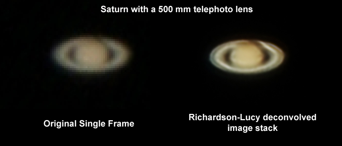
Figure 1. The planet Saturn imaged with a 500 mm f/4 telephoto lens
with stacked 1.4 and 2x teleconverters on a Canon 10D 6-megapixel digital camera.
Total focal length = 1400 mm, at f/11.2 (125 mm aperture).
Exposure time was 1/20 second at ISO 400 on a stationary camera tripod and only jpeg
images were recorded.
On the left is a single frame. On the rights the deconvolved
image after stacking 99 frames. Image obtained on March 20, 2004.
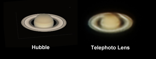
Figure 2. The planet Saturn imaged with the Hubble space telescope
(public domain image) and the deconvolved image with the Telephoto lens from Figure 1.
This comparison helps illustrate what is real in the deconvolved image.
The Hubble image has the rings slightly less open and there is less shadow
on the right side. But the Hubble shows the 3 main rings, from outer to inner
are the A-ring, separated by a dark band called the Cassini Division, then the middle
bright B ring and the faint inner C ring. The C-ring shows as a dark band in front of
the planet. All these features show in the telephoto deconvolved image and
are not apparent at all in the original single frame image in Figure 1.
The bands on the planet are different between the Hubble and telephoto images
because they were taken at different times.

Figure 3. The 99-image average (left) was run through unsharp mask with a couple
of different settings (middle) but the result is not as good as the Richardson-Lucy
image deconvolution (right). On top are 2x enlarged images and below the images
that were sharpened. Note the unsharp mask results show more noise than
the Richardson-Lucy results.
Sharpening Details
The 99 single images, each a 1/20 second exposure (Figure 1, left) and recorded as a jpeg
were graded and a weighted average made using tools in ImagesPlus (Figure 3, left)
and a 16-bit tif image files was written to disk. The 16-bit tiff file can be downloaded
here (file saturn.avg-mgraded.v1.0-r120.tif 1.5 MBytes).
Try your own method; I'll be interested to see your results if you can match and/or
surpass the image in Figure 1 (right side).
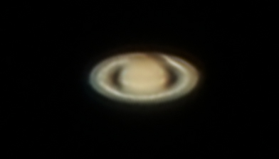
Figure 4. First Richardson-Lucy
image deconvolution attempt.
The image detail was improved
using Richardson-Lucy adaptive restoration: 10 iterations with a 9x9 box,
then 70 iterations with a 7x7 box using ImagesPlus, then final stretching (a small tweak) in Photoshop.
Plate scale on the large images is 4x the original = 0.27 arc-second
per pixel. Hints of the Cassini Division, a dark gap separating the
outer slightly fainter "A" ring from the Brighter "B" ring is seen
in the deconvolution in Figure 4. The Cassini Division is about 0.8
arc-second wide. The diffraction disk diameter is 2.2 arc-second for
the 125 mm lens, and the Dawes limit (~0% MTF) is 1.1 arc-second. Thus,
the adaptive Richardson-Lucy deconvolution improved image resolution to
a little better than the Dawes limit (better than 0% MTF). The total
improvement in spatial resolution is on the order of 3 times.
The second try pushed a little harder and resulted in the deconvolved image
in Figures 1 (right), 2 (right), and 3 (right). This image was produced
Richardson-Lucy deconvolution using Gaussian point spread functions
with 9x9 Gaussian, 40 iterations, followed by 7x7 Gaussian
and 150 iterations. The image was then stretched in photoshop using
curves. No additional sharpening was applied (e.g. unsharp mask).
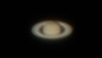
Figure 5. Image from Figure 3, left after Richardson-Lucy deconvolution
using a 9x9 Gaussian point spread function, with 40 iterations.
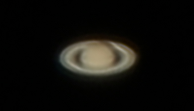
Figure 6. Image from Figure 5 after Richardson-Lucy deconvolution
using a 7x7 Gaussian point spread function, with 150 iterations.
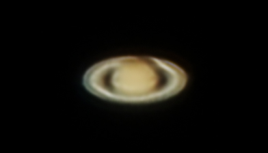
Figure 7. Image from Figure 6 after image stretching.
Conclusions
It is pretty clear that image deconvolution methods can increase resolution and produce
much sharper images than simple edge enhancement methods like unsharp mask.
The approximately 3x improvement in resolution is made possible by the high
signal-to-noise ratio image. Lower signal-to-noise ratios will result in
less improvement before noise is enhanced too much for many viewer's tastes.
The image used here was made with an early generation digital camera in 2004.
With modern digital cameras having lower noise, and by recording raw data,
which would also reduce noise, many fewer frames would be needed to
produce the same result.
The iterative deconvolutions were done using an intel I7-950 cpu running at
3.07 GHz. The iteration runs took a under about a minute for each set.
The original runs done for the first version of this article were made on
a much slower machine and took many minutes. With today's fast
desktop and laptop computers, advanced deconvolution methods can be
completed in reasonable time.
If you find the information on this site useful,
please support Clarkvision and make a donation (link below).
This is part 3 of illustrating image sharpening methods.
Part 3 is
here: http://clarkvision.com/articles/image-restoration3/.
Image Sharpening Introduction:
http://clarkvision.com/articles/image-sharpening-intro/
Part 1 is
here: http://clarkvision.com/articles/image-restoration1/
Part 2 is
here: http://clarkvision.com/articles/image-restoration2/
This page URL:
http://clarkvision.com/articles/image-restoration3
First Published March 19, 2005
Last updated February 16, 2014