Canon 1D Mark II Review and Sensor Analysis
Plus Procedures for Evaluating Digital Camera
Sensor Noise, Thermal Noise, Dynamic Range, and Full Well Capacities
by Roger N. Clark
This review shows an analysis of noise, dynamic range, and full well capacity
of a Canon 1D Mark II digital camera.
It also shows the dark current and noise from thermal
dark current as a function of temperature.
All images, text and data on this site are copyrighted.
They may not be used except by written permission from Roger N. Clark.
All rights reserved.
If you find the information on this site useful,
please support Clarkvision and make a donation (link below).
How well do digital cameras perform? On this web page, I'll
show the details on how to evaluate the sensor in a digital camera.
Using simple models one can test various possible noise
sources in a camera system. The lowest possible noise from a
system detecting light is the noise due to Poisson statistics
from the random rate of arrival of photons. This is called
photon statistics, or photon noise. Noise from the electronics
will add to the photon noise. We will see that
the Canon 1D Mark II is limited by photon statistics at high
signal levels and by electronic noise from reading the sensor
(called readout noise) at very low signal levels.
In the case of high signal levels, a system that is photon statistics
limited enables us to directly measure how many photons
the sensor captures, and by increasing the exposure, we can
determine how many photons are required to saturate the
sensor. That is called the full well capacity.
In order to analyze a camera, one needs appropriate data. This is
very simply done. Here are the steps.
The challenge in analyzing noise and full well capacities of a
camera sensor is obtaining data that is free of artifacts.
Artifacts could include non-uniformity of the light field
(e.g. due to vignetting in the lens), dust specs on the sensor,
pixel to pixel sensitivity variations and other effects.
Fortunately, there is a simple way to neutralize these effects.
If you take pairs of images at the same exposure and in rapid
succession, then difference the two images, the residuals
for a quality sensor is the noise due to electronics plus
photons. Light variations are eliminated. But one should
try and make a uniform setup in order to drive all pixels
at very close to the same light level.
Experiment Setup
I chose a uniformly lit wall in a room with mostly white
walls. I chose a room with multiple lights plus sunlight coming
in through a window. I put a 180mm f/3.5 lens on the camera
and mounted it on a tripod. I focused the lens to
infinity and placed the lens about a half meter from the
wall. This setup ensures the wall is out of focus,
and that a small portion of the wall is in the field, so
a reasonably uniform signal illuminates the sensor.
Obtaining the Data Set
Set the camera to its lowest ISO setting.
I first metered the scene
to see what a good exposure would be. I then
set the camera on manual and took a series of
exposures in pairs. Exposures ranges from the
minimum the camera was capable of, to a long
enough exposure that all pixels were saturated
in all colors. The exposures I used ranged
from 1/8000 second to 0.8 second and I used
two f/stops (f/5.0 and f/5.6). There is no
need to vary the f/stop, but if you do you
can check the accuracy of the f/stops too.
At each exposure setting, two images are obtained
within a few seconds of each other. I waited
for the data to be written to the memory card
before doing the next exposure.
I did exposures pairs at both the lowest ISO setting,
and at a high setting, in this case ISO 1600.
Only the ISO 50 data are presented here.
A second set of data tests read noise. Put the lens
cap on the camera and set the exposure time
to the maximum the camera will do (1/8000 second
for the 1D Mark II). For each ISO setting,
take a pair of exposures. I did ISO 50,
100, 200, 400, 800, 1600, and 3200.
Here is a more complete write-up on taking the data:
How to Take the Data .
Data Processing
The procedure below is based on using ImagesPlus 2.5,
hereafter called IP. The image
processing system you use must be able to convert the raw
data with a linear scale (Photoshop will not do this) and
process the data with at least 16-bit math (IP
uses 64-bit floating point math).
- Raw conversion: convert with no white balance, select CFA.
Save the images in either 16-bit tiff or compressed FIT
(I use lossless compressed FIT as it saves a lot of disk space).
An excellent raw converter (free) is dcraw. Convert the
raw files with: dcraw -D -4 -j -t 0 -T rawfilename and this
makes a tif file.
- Split the Bayer CFA (this is under the color menu).
I open all images in IP, then open the split Bayer CFA
window. Select each image, click apply and the red, green
and blue images will be created. Click on each image,
and save (confirm the over-write or the image will go away
later), then close each one after saving.
- I move the red, green, and blue images to their own
subdirectories for processing.
- Next, cd to the green directory, and crop the files.
I crop about the center (default) with width and height
of 200 pixels each. This is done as one step in IP
under files, image file operations, crop files.
- Open a pair of cropped images done at the same exposure.
Also open the cross hair statistics tool. The tool gives
the average intensity and standard deviation for the entire image.
Record the average intensity for each image.
- Now subtract the the two images with the image math
tool (under the point menu). To do this, open the
image math tool, then click the select source 1 box,
then click on one of the two images, then select
the other source box and click on the other image.
The images are 16-bit unsigned integers, so you must
do a trick to make sure the subtraction does not go
below zero. Under source 2, type in an offset
of 1000 or 2000, or more. The value does not matter,
except you want to be sure that the subtraction does
not go below zero. Click the subtract button and
the subtracted image is created. The cross hair
statistics tool will show the standard deviation,
minimum and other statistics. Be sure the minimum
is above zero. If not, increase the offset and
click subtract again in the image math window.
The standard deviation represents the noise in
TWO images. The noise in one image is square
root 2 less, so divide the standard deviation
by root 2 (1.4142) and record that value for both
images.
Results
Results for determining read noise is shown in Table 1a. Column B is the standard
deviation from subtracting two images, and Column C = column B / 1.4142.
Column D = column C / 16 which scale the 16-bit DNs to camera 12-bit DNs.
Column E is the gain derived from data in Table 2 by dividing the high signal in
electrons by camera DN. Gains at ISOs higher than 50 are scaled relative
to that at ISO 50 (this scaling agrees within the noise of determining gains
at each ISO). Read noise, Column F = Column D * Column E.
Dynamic range, Column G = maximum signal / read noise. Maximum signal
is 79,900 electrons (Table 2) at ISO 50, and 53,000 electrons at ISO 100.
Higher ISO reduces the maximum electrons relative to ISO 100 (e.g. ISO 200
is half the electrons of ISO 100). Column H is the square root of the number of
photons recorded (e.g. square root 79,900 at ISO 50; square root 53,000 at
ISO 100).
Table 1a: Canon 1D Mark II Read Noise and Dynamic Range
| A | B | C | D | E | F | G | H |
| ISO |
2-image
16-bit
Std Dev
DN
| 16-bit
Std Dev
per pixel
(DN) | Camera
noise
Std Dev
(12-bit DN) | Camera
Gain
(12-bit)
(electrons/DN)
|
Read Noise
(electrons) |
Dynamic
Range |
Maximum
Signal-to-Noise
ratio |
| 50 |
26.618 | 18.822 | 1.176 | 26.03 | 30.62 |
2610 | 283
|
| 100 |
28.871 | 20.415 | 1.276 | 13.02 | 16.61 |
3190 | 230
|
| 200 |
31.104 | 21.994 | 1.375 | 6.51 | 8.95 |
2960 | 163
|
| 400 |
38.686 | 27.355 | 1.710 | 3.25 | 5.56 |
2380 | 115
|
| 800 |
56.219 | 39.753 | 2.485 | 1.63 | 4.04 |
1640 | 81
|
| 1600 |
108.604 | 76.795 | 4.800 | 0.81 | 3.90 |
850 | 58
|
| 3200 |
218.527 | 154.522 | 9.658 | 0.41 | 3.93 |
420 | 41
|
Using data from the analysis here, the sensor performance is summarized in
Figure 1b. The gain (Table 1b, column B) reaches unity at about ISO 1300.
Once gain drops below 1 electron/DN, there is little point in increasing ISO
further. The effect of higher ISO above unity gain only decreases
dynamic range without helping to detect lower signals.
Table 1b: Canon 1D Mark II: Derived Sensor Performance
 A        B            C          D         E        F         G
        Camera     Apparent
ISO      Gain     Read Noise   Maximum   Dynamic  Dynamic    Maximum
     (electrons/  (electrons)  Signal     Range    Range  Signal-to-Noise
      12-bit DN)             (electrons) (linear) (stops)     Ratio

  50    26.03        30.62     79,900    2,610     11.3       283
 100    13.02        16.61     53,000    3,190     11.6       230
 200     6.51         8.95     26,500    2,960     11.5       163
 400     3.25         5.56     13,200    2,380     11.2       115
 800     1.63         4.04      6,620    1,640     10.7        81
1600     0.81         3.90      3,310      850      9.7        58
3200     0.41         3.93      1,650      420      8.7        41
The camera noise statistics are shown in Table 2. The normalized
exposure time, Column B, normalizes the changes in f/stops used during
the test (f/5.0 and f/5.6). The average DN, Column C, is the average
signal observed in a 200 x 200 pixel patch in the center of the image.
A model was constructed to check system linearity, Columns D and E.
The model in Column D = (3354.27 * Column B/0.4)-7. The constant
3354.27 is the average signal for image JZ3F7540, and the constant 7
represents an offset in the electronics to keep the signal level above 0.
The constant 0.4 scales the exposure time relative to that of the
reference image, JZ3F7540.
The system linearity, Column E = Column C / Column D, and is within a few
percent, which is very good. System linearity includes the detector
linearity, shutter reproducibility, f/stop reproducibility, and light
source stability. Note in the shorter shutter speeds, the signal
level in pairs of exposures varies a small amount. This was traced
post experiment to a nearby fluorescent light that contributed a high
frequency flicker to the light signal. That light is at least partly
responsible for the variable signal levels at a few percent level in
short exposures. That would not effect noise determinations, however.
The lesson is check all light sources and be sure only incandescent
lights contribute to the signal.
Pairs of the same exposure time and f/stop were subtracted and the
standard deviation divided by square root 2 is shown in Column F of Table 2.
The signal-to-noise ratio, Column G, is the values in Column F divided
by those in Column C. If the sensor is photon noise limited, the trend
in this ratio is a square root dependence. There are several ways
to determine the number of converted photons (the number of electrons)
from the sensor. A common way is to evaluate sensor noise is to
plot the variance versus signal (References 1, 3).
That is a straight line if the system is photon noise limited and the
slope of the trend represents the gain in electrons/DN, and similar a trend
line is shown in Figure 3 from data in Column I. While both methods
are equally valid, I prefer analyzing the signal-to-noise ratio because
that ratio squared directly equals the number of photons collected
without needing gain conversions, or computing the slope of a line.
So, is the Canon 1D Mark II photon noise limited? Column H shows a model
that uses the read noise from Table 1 (30.62 electrons at ISO 50) and the
Signal to noise ratio derived from the model from Table 2, Column D and
the system gain. The equation is:
H = (D*26.03/16)/(sqrt(D*26.03/16 + 30.62*30.62)), (eqn 1)
where the letters H and D are the values in Columns H and D in Table 2.
The value 16 scales 16-bit Column D DNs to Camera 12-bit DN to match
the units of the gain, 26.03 electrons/12-bit camera DN.
The Canon 1D Mark II signal-to-noise ratio data and model (Columns G and H in
Table 2) are plotted in Figure 2. The fact that the model matches the data
very well indicates there are no other sources of noise contributing to
the data at any significant level. Thus, for high signal levels, the 1D Mark II
is photon noise limited. This means further improvements in electronics
will not improve the signal-to-noise ratio for high signal levels. If the quantum
efficiency were improved with a different sensor, that would certainly improve
the signal-to-noise ratio.
Table 2: Canon 1D Mark II Noise Statistics
   A          B           C        D        E        F      G         H          I
          Normalized           Predict  Linearity   Noise           Predicted
          Exposure    Average  norm to  DN/Predict  Std dev Signal/  signal/   Signal
File Name time (sec)    DN     JZ3F7540    (%)       (DN)    noise   noise   (electrons)
JZ3F7568  0.000125      14.54     10.49   27.86    16.939    0.859    0.552      0.74
JZ3F7569  0.000125      16.00     10.49   34.41    16.939    0.944    0.552      0.89
JZ3F7566  0.000376      20.61     24.47  -18.75    19.597    1.052    1.274      1.11
JZ3F7567  0.000376      27.59     24.47   11.30    19.597    1.408    1.274      1.98
JZ3F7564  0.000627      47.83     45.46    4.96    23.015    2.078    2.325      4.32
JZ3F7565  0.000627      55.83     45.46   18.58    23.015    2.426    2.325      5.88
JZ3F7562  0.001254     112.05     97.91   12.62    24.491    4.575    4.810     20.93
JZ3F7563  0.001254     124.03     97.91   21.06    24.491    5.064    4.810     25.65
JZ3F7560  0.002509     218.37    202.83    7.12    25.909    8.428    9.268     71.04
JZ3F7561  0.002509     249.63    202.83   18.75    25.909    9.635    9.268     92.83
JZ3F7558  0.005018     490.64    412.65   15.90    28.527   17.199   16.737    295.81
JZ3F7559  0.005018     362.52    412.65  -13.83    28.527   12.708   16.737    161.49
JZ3F7556  0.007903     737.39    653.95   11.32    32.054   23.005   23.781    529.22
JZ3F7557  0.007903     673.15    653.95    2.85    32.054   21.001   23.781    441.02
JZ3F7554  0.016307    1518.77   1356.86   10.66    39.798   38.162   39.362   1456.33
JZ3F7555  0.016307    1371.70   1356.86    1.08    39.798   34.466   39.362   1187.94
JZ3F7552  0.031360    2914.53   2615.81   10.25    50.681   57.507   59.053   3307.07
JZ3F7553  0.031360    2880.75   2615.81    9.20    50.681   56.841   59.053   3230.86
JZ3F7550  0.062720    5867.70   5238.63   10.72    68.842   85.235   87.624   7264.93
JZ3F7551  0.062720    5826.18   5238.63   10.08    68.842   84.631   87.624   7162.48
JZ3F7527  0.100000    8530.99   8356.57    2.04    81.014  105.303  112.774  11088.67
JZ3F7528  0.100000    8585.31   8356.57    2.66    81.014  105.973  112.774  11230.33
JZ3F7548  0.096589    9361.93   8071.27   13.79    84.383  110.945  110.706  12308.86
JZ3F7549  0.096589    9277.50   8071.27   13.00    84.383  109.945  110.706  12087.85
JZ3F7529  0.125000   10701.77  10447.46    2.38    89.257  119.898  126.918  14375.50
JZ3F7530  0.125000   10765.38  10447.46    2.95    89.257  120.611  126.918  14546.90
JZ3F7531  0.167000   13553.07  13960.16   -3.00   100.351  135.056  147.686  18240.23
JZ3F7532  0.167000   13595.36  13960.16   -2.68   100.351  135.478  147.686  18354.24
JZ3F7533  0.200000   17081.52  16720.14    2.12   111.442  153.277  162.158  23493.84
JZ3F7534  0.200000   17087.82  16720.14    2.15   111.442  153.334  162.158  23511.18
JZ3F7535  0.250000   21440.86  20901.92    2.51   124.005  172.904  181.913  29895.70
JZ3F7536  0.250000   21495.32  20901.92    2.76   124.005  173.343  181.913  30047.77
JZ3F7537  0.300000   26751.08  25083.70    6.23   137.544  194.492  199.729  37827.01
JZ3F7538  0.300000   26737.60  25083.70    6.19   137.544  194.394  199.729  37788.89
JZ3F7539  0.400000   33584.17  33447.27    0.41   148.920  225.518  231.285  50858.30
JZ3F7540  0.400000   33454.27  33447.27    0.02   148.920  224.646  231.285  50465.64
JZ3F7541  0.500000   41632.24  41810.84   -0.43   159.079  261.709  259.029  68491.47
JZ3F7542  0.500000   40733.26  41810.84   -2.65   159.079  256.058  259.029  65565.48
JZ3F7543  0.600000   49136.00  50174.41   -2.11                              79938.13
JZ3F7544  0.600000   49136.00  50174.41   -2.11                              79938.13
JZ3F7545  0.800000   49136.00                                                79938.13
JZ3F7546  0.800000   49136.00                                                79938.13
Figure 1. The Canon 1D Mark II shows a very linear trend with signal.
Variations in signal level include repeatability of the shutter and aperture,
as well as the light source.
The model is the average DN from image JZ3F7540 scaled according to exposure
time and subtract 7 DN.
Figure 2. Signal-to-noise ratio observed and predicted. The prediction
model uses photon statistics and read noise.
Model is average DN scaled to electrons plus read noise. For this case,
ISO 50, the gain is 26.03 electrons/DN, and the read noise is 30.62 electrons.
Figure 3. The electrons converted by the canon 1D Mark II sensor
are shown relative to exposure level. The sensor saturates at about
79,900 electrons, but is quite linear below that level.
Noise Sources
The "read noise" in Tables 1a and 1b vary with ISO and have been
a source of confusion to phtographers reading these results.
The analog-to-digital converter (A/D, or ADC) used in the Canon 1D Mark II
is 12-bits. Noise specifications for typical 12-bit A/Ds running
in the tens of megahertz range are expressed in decibels (dB)
and typically give about a 70 dB signal-to-noise ratio.
Twelve bits if perfect would give 72.2 dB (=20 log(4095)), so
70 dB is very good. In Figure 4, the noise floor is modeled as
a function of ISO, using the data in Table 1a. Only 2 noise sources
are needed to model the observed noise: a base level of sensor read noise
that is constant at all ISOs, and a constant 70.5 dB of
noise-to-noise ratio from the
A/D converter. This illustrates that newer cameras employing
14-bit converters should have improved performance at low
ISO. The Figure also illustrates one should use ISOs of 800 or higher
for low light work, because the noise is dominated only by sensor
read noise.
Figure 4. Camera noise sources for fast shutter speeds
are well modeled with only two sources: sensor read noise and
noise from the analog-to-digital converter.
The noise model is the square root of the sum of the squared
noise sources (A/D signal-to-noise ratio = 70.5 dB
and the sensor read noise =3.8 electrons).
The observed noise are the values from Table 1a, column F.
Dark Current and Related Noise
Another noise component is due to dark current, which will
increase with exposure time. Dark current and its noise is
also a function of the temperature of the sensor and associated
electronics.
Dark current was measured at room temperature for 623 and 1800 second
exposures at ISO 1600. Pairs of images were analyzed similar to that
done for read noise. There is not a clean answer because as exposure time
increases, dark current for each pixel is obviously quite variable,
resulting a large variation in signal. Long exposure images look
like they have a lot of noise spikes. Average dark currents were
measured at 0.013 to 0.02 electrons/second, but some pixels have
dark currents as high as about 0.25 electrons/second. In an 1800 second
exposure, that translates to signal levels of 23 to 450 electrons,
and noise of 5 to 21 electrons. It is this pixel to pixel
variation that limits the image quality of long exposures (Figure 4).
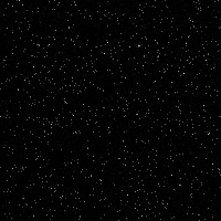
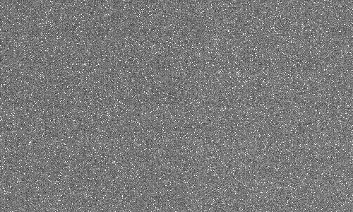
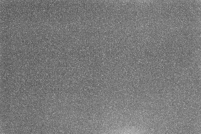
Figure 4. The noise in a 1D Mark II image is shown in this cropped
portion at full scale (1 camera pixel to 1 image pixel) for an
1800 second exposure at ISO 1600. Linear raw conversion in ImagesPlus 2.5.
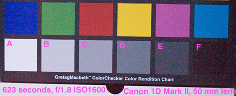
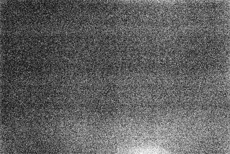
Figure 5. A 623 second exposure of a target illuminated by only
0.00016 lux. The 1D Mark II camera was operating at room temperature
and ISO 1600 with a 50mm f/1.8 lens. This image has had no stretching
or processing other than raw image conversion in photoshop
with default settings, then the two rows cropped
from the full image and downsampled about 4x.
The width of the image is the full height of the original image.
The tilt of the target was intentional so image edges did not line up
with rows of pixels.
A test of a long exposure is shown in Figure 5. The 623 second exposure
at ISO 1600 shows some noise but is generally a very good image considering
the illumination was only 0.00016 lux (similar to an overcast night
away from cities with no moon; it took several minutes of dark adaption to
to begin to see the target in the room). The light detected is shown in
Table 3 along with the noise analysis and model prediction.
Table 3: Color Target Noise Statistics
Color
Chart
Patch |
Average
Intensity
(Photons) | Photon Rate
(Photons per
pixel/second)
| Measured
Noise
(electrons) | Noise
Model
(electrons) |
| A | 749.4 | 1.21 | 26.9 | 30.3 |
| B | 494.9 | 0.794 | 24.0 | 25.8 |
| C | 288.7 | 0.463 | 22.7 | 21.4 |
| D | 148.5 | 0.238 | 21.4 | 17.9 |
| E | 60.6 | 0.097 | 21.2 | 15.2 |
| F | 19.4 | 0.031 | 16.8 | 13.8 |
The data in Table 3 shows that DSLRs like the 1D Mark II can operate at
very low light levels at room temperature. The noise model is:
N = (P + r2 + t2)1/2, (eqn 2)
Where N = total noise in electrons, P = number of photons, r = read noise
in electrons, and t = thermal noise in electrons. Noise from a stream of
photons, the light we all see and image with our cameras, is the square root
of the number of photons, so that is why the P in equation 2 is not squared
(sqrt(P)2 = P). The model used the read noise of 3.9 electrons from
Table 1. The thermal noise squared = the dark current = 0.25 electrons/second * 623 seconds
= 157.75 electrons2.
Similar noise models are discussed in reference 6.
Pattern noise in long exposure dark frames is shown in Tables 4a, 4b and 4c.
| Table 4a. Thermal Noise, Central Image |
 |
ISO 1600
Exposure= 623 seconds
T= 20 C
Image Range:
-100.00 to 100.00 electrons about the mean
Central 500 x 300 pixel statistics:
min= 21 electrons
max= 3006 electrons
mean= 104 electrons
standard deviation= 48.77 electrons |
| Table 4b. Thermal Noise, Full Image, sub-sampled |
 |
ISO 1600
Exposure= 623 seconds
T= 20 C
Image Range:
-100.00 to 100.00 electrons about the mean
Full image statistics:
min= 6 electrons
max= 3006 electrons
mean= 106 electrons
standard deviation= 50.76 electrons |
| Table 4c. Thermal Noise, Full Image, sub-sampled |
 |
ISO 1600
Exposure= 623 seconds
T= 20 C
Image Range:
-20.00 to 20.00 electrons about the mean
Full image statistics:
min= 6 electrons
max= 3006 electrons
mean= 106 electrons
standard deviation= 50.76 electrons |
Conclusions
The data shown here for the Canon 1D Mark II shows that the camera is
operating and near perfect levels for the sensor. This means that for
high signals, noise is dominated by photon statistics. Noise at low
signal levels can be improved, but is very good. To achieve higher
signal-to-noise ratio images, a higher quantum efficiency sensor with
a larger full well would be needed. Without increasing the full well
capacity, the maximum signal-to-noise ratio would not improve, but that
the signal-to-noise ratio at ISO 50 could be achieved at higher
ISOs if the quantum efficiency were improved. Improvements in quantum
efficiency of 3 to 4x are possible (Reference 2).
The data for the 1D mark II indicate some important aspects for people
making images. The lowest ISO, 50, does have higher signal-to-noise ratios
than ISO 100, but at the expense of lower dynamic range and danger of
saturating highlights. An ISO of about 75 would be a better match
to the sensor range and would not sacrifice dynamic range. Unfortunately,
ISO 75 is not available.
For low light imaging, high ISO will record fainter light. There is no
advantage in using ISO 3200 and in fact there is a disadvantage in reduced
dynamic range. ISO 1600 is the optimum with the lowest read noise, but
ISO 800 is almost as good (almost the same read noise as ISO 1600) with
the advantage of almost double the dynamic range of ISO 1600.
Long exposures suffer from dark current that varies over a factor of
ten from pixel to pixel, ultimately limiting image quality of long
exposures. If dark current could be made more uniform, much longer
exposures could be made with high image quality. Even so, 10+ minute
exposures at ISO 1600 still produce acceptable images, recording
only a few photons.
With the details of how to evaluate sensor noise presented here, everyone
can evaluate their own cameras. For other descriptions, see References
1 and 3.
If you find the information on this site useful,
please support Clarkvision and make a donation (link below).
References
1)
CCD Gain. http://spiff.rit.edu/classes/phys559/lectures/gain/gain.html
2)
Charge coupled CMOS and hybrid detector arrays
http://huhepl.harvard.edu/~LSST/general/Janesick_paper_2003.pdf
3)
Canon EOS 20D vs Canon EOS 10D and
Canon 10D / Canon 20D / Nikon D70 / Audine comparison
http://www.astrosurf.org/buil/20d/20dvs10d.htm
4)
http://www.photomet.com/library_enc_fwcapacity.shtml
5)
Astrophotography Signal-to-Noise with a Canon 10D Camera
http://clarkvision.com/astro/canon-10d-signal-to-noise
6)
Concepts in Digital Imaging Technology
CCD Noise Sources and Signal-to-Noise Ratio
http://learn.hamamatsu.com/articles/ccdsnr.html
7)
dcraw. http://www.cybercom.net/%7Edcoffin/dcraw
8)
dcraw manual page.
9)
dcraw downloads.
Notes:
DN is "Data Number." That is the number in the file for each
pixel. I'm quoting the luminance level (although red, green
and blue are almost the same in the cases I cited).
16-bit signed integer: -32768 to +32767
16-bit unsigned integer: 0 to 65535
Photoshop uses signed integers, but the 16-bit tiff is
unsigned integer (correctly read by ImagesPlus).
http://clarkvision.com/reviews/evaluation-1d2
First published July 8, 2007.
Last updated January 18, 2014