Dynamic Range and Transfer Functions of Digital Images
and Comparison to Film
(Intensity Detail of Images)
by Roger N. Clark
All images, text and data on this site are copyrighted.
They may not be used except by written permission from Roger N. Clark.
All rights reserved.
The ability of a camera system to record a wide dynamic range and show
details throughout the dynamic range is very important to image quality.
How well do various system do? On this page, I test a Pro digital SLR camera,
professional slide film, and consumer print film as well as raw versus
jpeg images from the digital camera.
I constructed a test target, Figure 1, below that has a large range
of intensities. Spot metering shows the target had a dynamic range of
1500, or 10.6 stops (Figure 2).
All images were processed identically.
Quantitative results were derived from original unprocessed
data except for conversion (raw 12-bit file from the digital camera
converted to 16-bit linear tif image; raw 12-bit linear scans from
film written to 16-bit tif file).
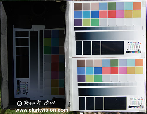
Figure 1. The test target consists of color blocks, gray blocks, and gray
ramps in intensity. The charts were printed, and one was placed inside
a box painted black to simulate detail in shadows. In the deep shadow
in the box above the test chart is a black tube, here called the "black
hole" which reflects almost no light. In this view, sunlight is illuminating
the target from the upper right. This image is from the Canon 1D Mark II
digital camera.
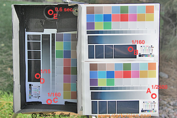
Figure 2. Example spot metering values on the test target. The shadows
have been enhanced in this image from Figure 1 using the Photoshop shadow tool, applied
twice: 100%, then 50%. The exposure times are for f/5.6 at ISO 100,
and range from 0.6 seconds in the "black hole" to 1/2500 second on the
white paper.
The image in Figure 1 was obtained with a Canon 1D Mark II camera in
raw mode and converted to a 16-bit tif file using Canon's software
with default settings. Two film types were also tested. Images of
the target with film and digital were interspersed by using 3 cameras
and one tripod. Time between images was less than a minute and repeated
several times to ensure any change in lighting was not an issue concerning
the results. The film was scanned on a sprintscan 4000 scanner at 4000
dpi using linear 12-bits, outputting a 16-bit tif file using standard settings.
The film images were registered to the digital camera images for detailed
comparisons. The film was developed at a professional lab, Reed Photo
in Denver, using standard developing.
An image of the test target on Kodak Gold 200 print film is shown in
Figure 3, and an image on Fujichrome Velvia ISO 50 slide film is shown
in Figure 4. It should be immediately obvious that the Fujichrome
Velvia image shows higher contrast, and except for a blue color cast
on the royal gold film, it has contrast similar to the digital image.
The highlights are similarly recorded in all three tests (digital,
print film, and slide film), and have intensities in the very bright
regions in the digital file within 4% of each other. Some portions
of the test images were driven to saturation. To do this, a series
of 15 exposures were recorded as a function of exposure time, both
above and below the metered exposure and the ones selected had the same
brightness at the high end for the same locations on the test target.
The exposure times were: Fujichrome velvia: 0.0 stop, 1D Mark II digital:
+0.3 stop, and the Kodak Gold 200: +1.0 stop from standard metering.
By selecting these exposures, the dynamic range from saturation to the
noise floor could be measured for each medium, and the three data sets
are registered at the bright end. This is why the curves in Figures 8
and 10 overlay each other at the high end (upper right in each Figure).
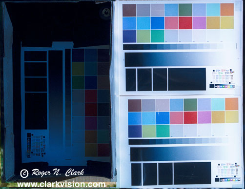
Figure 3. Image of the test target on Kodak Gold 200 print film.
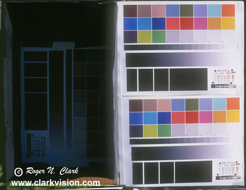
Figure 4. Image of the test target on Fujichrome Velvia, ISO 50. slide film.
The shadow detail of the three systems are shown in Figure 5. The images
have been stretched with the photoshop shadow tool by increasing the
shadow intensity 100% then another pass at 50%. Now we can see that
the digital images show much more shadow detail than either print
or slide film. Even an 8-bit jpeg digital camera image shows
more shadow detail than film.
Also of note: the print film shows More shadow detail than slide film.
The Fujichrome Velvia shows no hint of the "black hole," while the print
film barely shows it. The digital camera images show not only the
"black hole" but also more detail inside the box than either print or
slide film. Finally, the digital camera jpeg image has slightly more
noise than the raw image, but both show detail around the "black hole"
better than film. Note too, the jpeg image has a slight greenish cast
in the shadows. This can be corrected to some degree with processing,
as can the blueish cast of the Kodak Gold 200.
All this points to the digital camera having a larger dynamic range
than either print or slide film. This is not the commonly cited
wisdom. Now we will examine quantitative data.
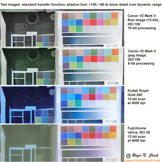
Figure 5. Comparison of shadow detail. The digital camera images show
more detail than either print or slide film. This is because of the
lower noise and larger dynamic range of digital camera images.
All images were processed identically. The shadows
have been enhanced in this image using the Photoshop
shadow tool, applied twice: 100%, then 50%.
The shadow detail in the film was confirmed visually by inspecting
the film under magnification: the scans show what can be detected
by visual inspection plus a little more.
Digital Transfer Functions
In order to quantitatively examine the dynamic range, transfer function,
and noise as a function of scene intensity, an image of the target was
converted to a 16-bit tif file with a linear conversion using the canon
1D Mark II data. The sensor is inherently linear, and spot metering
agrees with linear numbers derived from the 16-bit tif file over the
entire dynamic range. Traverses along intensity gradients were done
using ImagesPlus. For this work, 3 traverses were designed to cover
the entire dynamic range. Agreement in the overlap regions is good.
Figure 6 shows the transfer function of observed output intensity as
a function of scene intensity for the Canon 1D Mark II camera in raw
mode, with standard conversion using the Canon conversion software.
All intensities in this document are 16-bit values from the tif files.
Digital camera values are from 0 to 4095, so to get camera values,
divide by 16. A mix of linear and log scales will be used to illustrate
different points.
Figure 6. The Canon 1D Mark II standard processing of a raw file produces
these output intensities. Note for dark parts of the image, the scene
intensity is multiplied by 10. At low scene intensities (e.g. near 100),
spacing in the points every 16 DN is apparent because the original 0-4095
integers are multiplied by 16 to scale to the 16-bit tif file data range.
Next, let's compare jpeg versus raw output. This comparison is shown
in Figure 7 on a log-log scale. Here we see posterization of the
8-bit jpeg signal at low intensities. The larger scatter in the jpeg
data explains the slightly degraded shadow detail seen in Figure 5.
The horizontal banding of the red jpeg points is due spacing in multiples
of 256 because the 8-bit jpeg data were multiplied by 256 for comparison
with the 16-bit data.
Figure 7. Jpeg and raw Canon 1D Mark II digital camera transfer functions.
Note how the jpeg shows increased noise over the raw data.
Figure 8a, 8b, below, show the transfer function of a digital camera
(a Canon 1D Mark II) compared to print film (Kodak Gold 200), slide
film (Fujichrome Velvia), and the relative response of the Human eye
(note the human eye has a much greater dynamic range). What this
graph shows is that the digital camera response function is similar to
print film, but slightly lower in contrast in some parts of the curve, slightly higher
in other parts. Fujichrome Velvia has the highest contrast of the 4
systems shown. But also of interest is the noise. Note that the digital
camera points follow a nice smooth line. The Fujichrome Velvia points
follow a trend with scatter of individual points several times larger
than the digital camera until the signal is lost in noise (below about
scene intensity = 500 DN). The print film shows the widest scatter
and therefore has the highest noise. Also of interest is where each
curve flattens out in the lower left corner. Note the Fujichrome Velvia
slide film begins to flatten at about 3000 DN on the Scene Intensity,
and really flattens out just above 1000 DN. The print film flattens
out (and also becomes excessively noisy) below about 900 DN. But the
digital camera keeps going to the bottom end of the data below 70 DN.
Noise in the digital camera image over the "black hole" was measured
at 19 DN (note: that is 1.2 camera DN, limited by the A to D conversion).
The Kodak gold average signal keeps decreasing toward lower signal,
but the signal becomes lost in excessive noise. This shows that the Canon
1D Mark II has a much higher dynamic range than either Fujichrome Velvia
slide film and Kodak Gold 200 print film. Kodak Gold 200, in this test,
showed 7 stops of information, Fujichrome Velvia 5 stops, and the Canon
1D Mark II, over 10 stops of information! Further image analysis shows
at least 10.6 stops are recorded by the canon 1D Mark II camera (the full
range of of detail in this image, Other testing of the noise level versus
intensity shows the Canon 1D Mark II has 11.7 stops of dynamic range.
Figure 8a. Comparison of the Canon 1D Mark II digital camera response compared to
print film, slide film, and the human eye.
Figure 8b. Comparison of the Canon 1D Mark II digital camera response compared to
print film, slide film in photographic stops.
Raw versus Jpeg
Recall Figure 7 which showed a difference in noise between raw and jpeg
images. In Figure 9a, 9b, 9c, we zoom in on the data in Figure 7 to show
the details. In Figure 9a is shown detail for the brightest portions
of the scene. It is not necessarily important that the two curves do
not overlap. More important is the posterization of the jpeg data.
This is observed as the red points fall along short horizontal lines.
Their interval is 256 because of the scaling from 8 to 16-bit. The raw
data (blue points) show a more continuous curve and therefore more detail
in the highlights in the image.
Figure 9a. Jpeg versus raw transfer function and noise detail.
Figure 9b and 9c show the details of the jpeg versus raw data for mid-tones
in the image. While posterization is present, it is small in comparison
to the large range of intensities.
Figure 9b. Jpeg versus raw transfer function and noise detail.
Figure 9c. Jpeg versus raw transfer function and noise detail.
Figure 9d shows the intensity comparison between jpeg and raw data
for the darkest parts of an image. Posterization is apparent but
is masked somewhat by increased noise in the jpeg data.
Figure 9d. Jpeg versus raw transfer function and noise detail.
How do the transfer curves presented here compare to film Characteristic
Curves? Figure 10 compares Kodak's published data on the Characteristic
Curve of Kodak Gold 200 which the data for the same film derived in
this study. Within the scatter of the points in this study, the two
curves agree, and similar basic trends are observed. The film data for
this study was at a constant high resolution, so film grain dominates the
signal at low intensities. While the characteristic curve data shows
a signal could be seen over larger dynamic range going into the dark
portions of a scene, that signal would have to be of a large target so
many film grains were averaged. Small detail would be lost in the noise.
The digital sensor, however, has much lower noise in the dark portions
of the scene, by factors of 10 and more!
The Kodak Gold 200 data are from the green channel at:
Kodak Gold 200 Data Sheet and
Kodak Gold 200 Characteristic Curve
Figure 10. Comparison on Kodak Gold's Characteristic Curve with data
measured for this study. Note how the bottom of the characteristic
curve is dominated by noise (brown points) at high resolution of a 4000 pixel-per-inch
scan. The Characteristic curve from Kodak (red line) is an average response.
Conclusions
Digital cameras, like the Canon 1D Mark II, show a huge dynamic range
compared to either print or slide film, at least for the films compared.
Jpeg digital camera images suffer from posterization and the problem is
significant for highlights and darkest portions of an image.
Digital camera transfer functions, like that in the Canon 1D Mark II camera,
are similar to print film.
While digital cameras like that tested here show superior intensity detail
and signal to noise, slow speed films have higher spatial resolution.
See:
Film Versus Digital Executive
Summary.
Also, see the article Dynamic Range of an Image
which shows that real scenes can have over 10 photographic stops of
dynamic range (a factor of over 1000).
Then explore the article on
The Signal-to-Noise of Digital Camera
images and Comparison to Film.
Notes:
DN is "Data Number." That is the number in the file for each
pixel. I'm quoting the luminance level (although red, green
and blue are almost the same in the cases I cited).
16-bit signed integer: -32768 to +32767
16-bit unsigned integer: 0 to 65535
Photoshop uses signed integers, but the 16-bit tiff is
unsigned integer (correctly read by ImagesPlus).
Dynamic range is defined as maximum intensity / minimum intensity,
where intensity is scene radiance. For a sensor, like in a
digital camera, the minimum is usually limited by noise.
Thus the dynamic range that can be recorded by a sensor can
be smaller than actual scene dynamic range.
Posterization is the integer quantization of digital data. For example,
16-bit data has 65535 levels while 8-bit data has only 256 levels.
In the conversion from 16-bit (or 12-bit camera) data to 8-bit,
some information is lost.
The dynamic range of the image data shown above. e.g. Figure 8, has some additional
characteristics that should be noted. If one averages the pixels for the
film data, one can extend the trend beyond the 7 stops of range I cite above
for the print film, and 5 for the slide film. Thus one could argue for
a larger dynamic range. While this is true, the problem is the noise becomes
excessive. As a result, one may be able to distinguish coarse details,
but not fine detail. Thus effective spatial resolution drops when
the noise becomes excessive. Thus while one can claim 10 or more stops
of information are recorded, the information at the extremes is of little
use. The definitions I used here are consistent for digital as well
as film sensors. These conclusions are similar to other who have
studied this problem. For example, see the following reference
external to this site:
Photoshop for Astrophotographers,
Chapter 1 - Perceiving and Recording Light, Sample Section
Dynamic Range
http://clarkvision.com/articles/dynamicrange2
First published November, 2004.
Last updated July 3, 2005