ClarkVision.com
| Home | Galleries | Articles | Reviews | Best Gear | Science | New | About | Contact |
Astrophotography and Exposure:
What Can You Image with Various Exposures?
by Roger N. Clark
| Home | Galleries | Articles | Reviews | Best Gear | Science | New | About | Contact |
by Roger N. Clark
People new to astrophotography often ask what exposure does one need for astrophotography? Here is a guide and simple method to calculate exposure. Exposure is a combination of lens aperture area and exposure time.
The Night Photography Series:
Contents
Introduction
Exposure, CEF
Exposure, CEFA
Example Images versus Exposure
Sub-Exposure Length
Advantages and Disadvantages of Short Exposures
Light Pollution Effects
Discussion and Conclusions
References and Further Reading
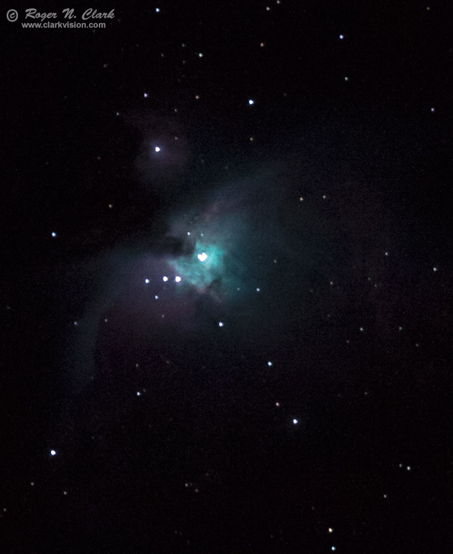
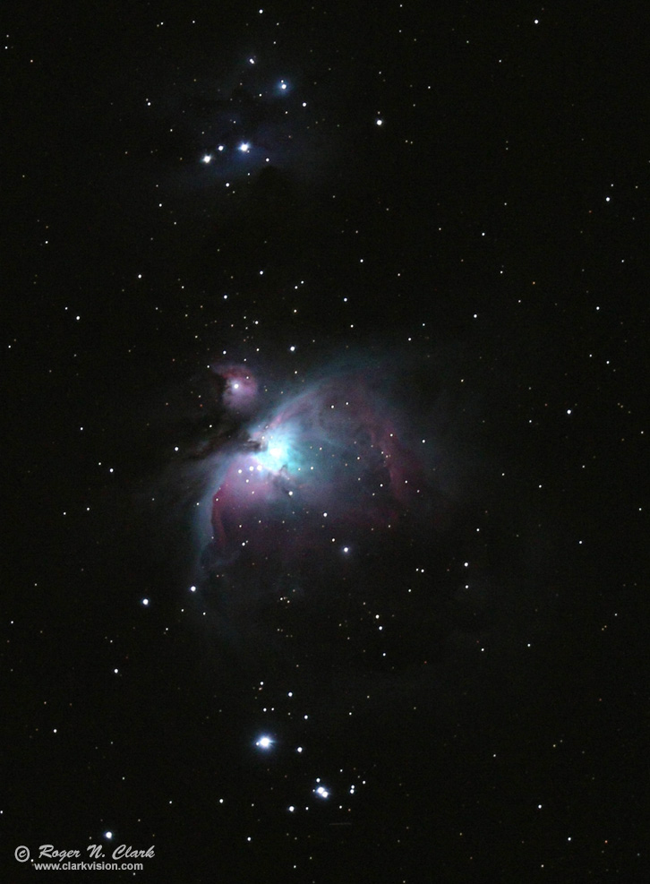
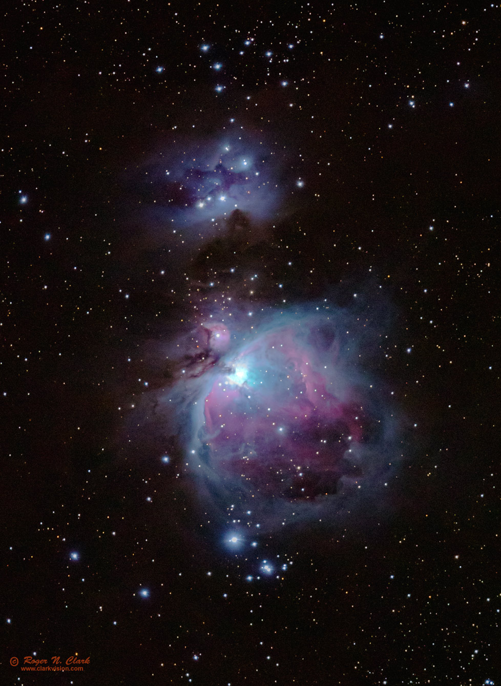
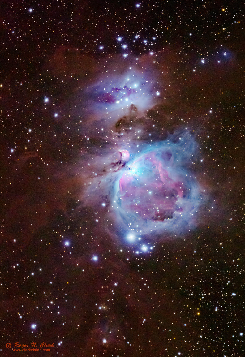
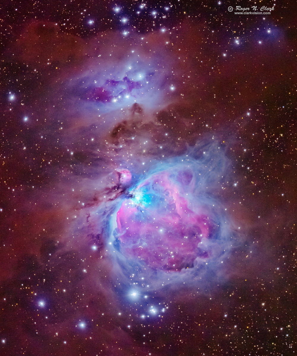
The page shows a series of images of The Great Orion Nebula, Messier 42, Messier 43 in the constellation Orion with increasing exposure using a 300 mm focal length lens and a 1.6x crop DSLR. One does not need a telescope to do a lot of astrophotography. Keys are fast lenses to collect a lot of light and a dark site away from cities.
Exposure in terms of light from the subject is the product of lens aperture area times exposure time. Exposure can be further refined by including angular area. This leads to two exposure factors that I have standardized on. 1) Clark Exposure Factor (CEF), and 2) Clark Exposure Factor Angular area (CEFA) Further, I standardize the units: aperture in square centimeters, exposure time in minutes, and angular area in square arc-seconds. There are other definitions of exposure factor (google: exposure factor photography), and other units can be used, but my definition uses specific units for direct comparison across a wide variety of conditions. Thus I call it the Clark Exposure Factor. Too be clear, this is basic, well-known physics, and I only add my name to indicate the units that I have standardized on. If you cite an exposure factor as a CEF please be sure to use the same units: minutes and square centimeters. If not, do not call it CEF.
Total light from the subject is key to the noise in a recorded image. The signal-to-noise ratio is the square root of the total light received from an object, whether daytime photography, or low light astrophotography, and is due do Poisson counting statistics. In a perfect imaging system, the signal-to-noise ratio we perceive in our images is the square root of the number of photons (light) collected by the sensor, and is called a photon-noise limited system. Other noise sources, e.g. noise from camera electronics, or noise from light pollution, add to the photon noise from the subject.
The basic physics is simple. For example, the light incident at the Earth's surface from a patch of nebula, or a star, will shine so many photons per square centimeter per minute on our telescopes/camera lenses/eyes. For example, consider a 10 arc-second square patch of the Orion nebula, The more square centimeters of light collection optics, the more light is collected per minute. The more minutes of exposure, the more total light from that patch. If two imaging systems, with different aperture diameters were exposed with different exposure times, the light collected from that patch would be the same if the aperture area times exposure time are the same. Then the noise will appear the same when the images are displayed at the same size. If they do not appear the same, then other noise sources are influencing the result, which may be due to noise in the camera electronics, quantum efficiency of the sensor, or transmission of the optics. If the images were made at different times and locations, noise from light pollution or airglow may be contributing to the differences. Most modern lenses/telescopes have similar and relatively high transmission. Most modern digital camera sensors have similar quantum efficiencies (about 50 to 60%). There is a larger range in dark currents from different sensors, and dark current can be a large factor in the noise in an image. Noise from dark current varies over a factor of 20 at the same temperature between modern sensors, and over a factor of 3,000 from -10 to +30 Centigrade when temperature effects are included. Noise from dark current is the square root of the dark current. So choosing a low dark current camera is important for very low light, long exposure imaging.
Below I show a series of images made with a 300 mm focal length lens. At 300 mm focal length, combined with excellent low light high megapixel digital cameras like the Canon 7D Mark II with 4.09 micron pixels records fine details in many deep sky objects. A 300 mm focal length lens with a camera with 4.1 micron pixels, resolves 2.8 arc-seconds per pixel. It is hard to actually record more detail than about 2 arc-seconds in long exposures due to atmospheric turbulence. Thus, it is rare that one would need focal length longer than about 600 mm with such cameras.
The Clark Exposure Factor is a measure of the relative amount of light received from a subject. It can be used to fairly compare wildly different lens/telescope apertures and exposure times.
Clark Exposure Factor, CEF = aperture area in square centimeters * exposure times in minutes
CEF = (pi/4) * (aperture diameter in cm)2 * time, pi = 3.14159.
For example, the image in Figure 1, a 1 second (1/60 minute) exposure was made with
a 300 mm f/2.8 lens, so the aperture diameter = 300/2.8 = 107 mm = 10.7 cm. Therefore, we
have:
CEF = (pi/4) *(30.0 cm/2.8)2 * (1/60 minutes) = 1.5 minutes-cm2.
Astrophotos made with the same CEF regardless of aperture and exposure time will be similar in image quality when made with approximately the same focal length (close to the couple of arc-seconds per pixel) and presented at similar sizes.
For widely varying focal lengths where you want to record a similar light density, include the pixel angular area. This is CEFA:
Clark Exposure Factor Angular area, CEFA = aperture area in square centimeters * exposure times in minutes
times angular area in arc-seconds.
CEFA = (pi/4) * (aperture diameter in cm)2 * time in minutes * angular area in sq. arc-seconds
The first step is to determine the angular size of a pixel, called the plate scale. See Plate Scale for details on the equations and tables for cameras and focal lengths.
Subject Plate Scale = 206265 * pixel pitch in mm / focal length in mm (result in units arc-seconds per pixel),
Where 206265 = the number of arc-seconds on one radian. The plate scale of a 300 mm lens
on a 7D Mark 2 with 4.09 micron (0.00409 mm ) pixels is:
Plate Scale (7D2 +300 mm) = 206265 * 0.00409 / 300 = 2.8 arc-seconds / pixel.
The pixel angular area is the square of the plate scale, 2.8*2.8 = 7.8 square arc-seconds.
For example, the CEFA for the image in Figure 1 is the CEF * pixel angular area
= 1.5 * 7.8 = 11.7 minutes-cm2-arc-seconds2.
Why is CEFA important? Say you saw the image in Figure 1, but wanted
to make a higher resolution image on a night of very steady atmosphere,
with imaging at 1-arc-second per pixel and a 150 mm diameter lens.
What exposure time would you need to get the same signal-to-noise ratio
per pixel? The image in Figure 1 has a 1/60 second
exposure time, so the CEFA with the 150 mm (15 cm) diameter lens in 1-second would be:
CEFA = (pi/4) *152 * (1/60 minutes) * 1 sq arc-second = 2.95 minutes-cm2-arc-seconds2.
Thus you would need 11.7 / 2.95 = 4 times longer exposure, or 4 seconds.
Note: CEFA is Etendue times exposure time.
The following images shown here were made with a Canon 7D Mark II 20-megapixel digital camera and 300 mm f/2.8 L IS II at f/2.8. No dark frame subtraction, no flat fields no bias were used. Tracking was with an Astrotrac but no guiding.
The images were made with daylight color balance. This is a stock camera with very close spectral response similar to the human eye. Astrophotographers often modify cameras for increased sensitivity to Hydrogen-alpha emission (red). The pink and light blue colors are close to what I have seen visually through large telescopes though a little more pastel. Hydrogen emission nebulae actually appear pink due to H-alpha (red), H-beta (blue) and emission from other atoms, like oxygen and sulfur. Modified cameras over emphasize H-alpha, making hydrogen emission nebulae come out red in photos. Unmodified cameras do a better job at color separation of the various processes that occur in the deep sky. Modified cameras tend to show mostly red in areas like that in this image, making it too difficult to tell the difference between dust and hydrogen emission nebulae. See Parts 2a - 2d of this series for descriptions of the natural colors in the night sky
The above exposure series used shorter exposures averaged together to achieve a given total integration time. To achieve detection of very faint light from stars, galaxies, nebulae, comets and other faint things in the night sky, one must minimize noise sources. The noise sources include:
Other factors also reduce efficiency when sub-exposures are short:
In making long exposures, the goal is to achieve a reasonable signal-to-noise ratio (S/N) and a sharp image. We can do that by using a large aperture lens/telescope. Noise from light pollution will be less if the light pollution is small, and you can make that happen by traveling far from cities, or use filters to block at least some of the light pollution (note that also blocks some light from the subject). Apparent read noise is a characteristic of a given camera. Apparent read noise generally decreases with increasing ISOs. Internet "experts" are generally obsessed with read noise, but it is relatively simple to make it insignificant by simply doing long enough exposures. Dark current noise is a function of temperature and generally doubles for every 5 to 6 degrees C increase in temperature. The only way to improve noise from dark current is to image on a cold night, do active cooling, or choose a camera with lower read noise (or all of these things).
To minimize the effects of read noise, simply expose long enough to get the histogram peak at about the 1/4 to 1/3 level on the camera LCD (Figure 6). Try and avoid the histogram peak going above the half way point as dynamic range can be impacted. This guideline works for read noise in the 2 to 4 electron range, which applies to most recent model digital cameras when used at ISOs around 1600. For lower read noise values, e.g. 1 to 2 electrons, lower histogram levels can be used without detrimental effects. More specifics are given below.
The histogram is a variable gamma scale and the 1/3 point means a signal at about 3% of full scale for the sensor. So if the sensor has a range of 2000 electrons maximum signal, that means the sky in the 1/4 to 1/3 histogram range would be about 60 electrons in that exposure, whatever length it might be. As you may surmise, with typical read noise below 3 electrons for modern digital cameras, the noise from the sky is much greater than the sensor apparent read noise (square root 60 = 7.7 which is obviously a greater number than 3. Some internet "experts" don't seem to understand this). So just keep your exposures long enough to get the histogram at the 1/4 to 1/3 level and you've done a good job of minimizing read noise contributions. What is more important is total exposure time. Once sub-exposure time reaches the 1/4 to 1/3 histogram level, longer sub exposure will not help, given the same long exposure time. Table 1 gives a guideline for dark site to very light polluted sites.
The above discussion argues for longer sub-exposure times. But there are factors that limit the length of sub-exposure times. These include:
Seeing is the bouncing around and blurring of the image due to atmospheric turbulence. The atmosphere may be stable for short periods, but then degrade with heat waves in the atmosphere between your camera and outer space. Shorter exposures can be selected to use only the images made in the most stable atmosphere periods. Random wind gusts can shake the imaging setup, moving the image around in the scene during exposures, burring the recorded image. The shorter the exposure, the higher the probably the exposure will complete before another wind gust. Tracking systems have periodic error and if you are not using an autoguider to correct this or you have slower drifts from polar alignment errors or drive rate errors, you are limited as to how long you can image before drift impacts image quality. Airplanes and satellites going through the image can be rejected using sigma-clipped averages if you have many frames to combine. If you have only a few frames, rejection of airplane and satellite trails are not well rejected and you must simply throw them out losing efficiency (or tediously clone them out after the stack). Try for at least 10 frames to combine (see Part 3e, Image Processing: Stacking Methods Compared) for methods to combine a set of images.
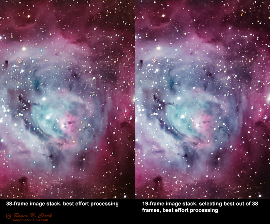
Videos showing the seeing effects in these two images is here in this dpreview thread.
Putting the above concepts together on dropping efficiency as sub-exposure length decreases, to lower efficiency as exposure times become longer due to seeing, wind, tracking, and interference from satellites and aircraft we get efficiency plots like that shown in Figures 8a, 8b, 8c. Even if your system has an autoguider and tracks perfectly, the other factors, like seeing still affect the final result.

Use these spreadsheets to tune the model for your systems and environmental conditions. The spreadsheets were created with libreoffice on linux, and I have tested both on a windows excel program. The xls file is probably best to use with windows and excel.
In using the model, you can look up the read noise and dark current for your camera, e.g. here. If you can't find dark current for your camera, estimate it from the blue and cyan lines in Figure 3 here. For the exposure time stability, first determine your total desired exposure time, say it is 100 minutes. Divide that by (approximately) 10 so that you have many sub-frames to stack and reject satellites and airplane tracks. That is the maximum sub-exposure time to consider. Next, what is the longest your mount can track a subject when you would reject a frame 50% of the time. If this is shorter than the minimum number of frames calculation, use this new number. Next is to evaluate environmental conditions: how long between wind gusts, and how long is the seeing stable? Use the shortest time from all these factors for the Exposer Time Stability factor.
The above model and example in Figure 7 clearly demonstrates that tuning sub-exposure length to best work with limitations of the system and environment can result in a better final image. Also Figure 7 illustrates that there are important factors in producing astrophotos than simply accumulating maximum exposure time. This means limiting sub-exposure length when seeing, wind, and tracking limits image quality and reject frames that are not sharp. If you end up rejecting many frames, that is reducing efficiency and in your next session, try shorter sub-exposure times.
Figure 8b shows model results for an older camera used at low ISO. The high read noise shifts peak efficiency to longer wavelengths. But note the efficiency is actually lower than with the lower read noise camera using shorter sub-exposures as shown in Figures 8a and 8c!
Some cameras are now in the 1-electron read noise range. Compared to the results in Figure 8a, we see the peak efficiency of the 1-electron read noise camera is shifted shorter to less than 1 minute. When sub-exposure times approach and become shorter than about a minute, the inter-frame delay to write results to the memory card become the major factor in efficiency. Use fast memory cards and reduce the delay time to the minimum. Be sure that the write cycle completes before the next exposure starts because the higher electronics activity can add noise to the next image if the camera is writing results during an exposure. For a Canon 7D Mark II, I use a 2-second delay for writing the image to a fast card, and 2-second mirror lock up delay, for an inter-frame delay of 4-seconds.
Technical. You can estimate the photons from the sky relatively simply for any modern camera. The maximum signal at base ISO for silicon photodiode sensors (that means CCDs and CMOS sensors in digital cameras) is about 2100 electrons per square micron. For example, the images above were made with a Canon 7D Mark II at ISO 1600 with 4.09 micron pixels, so it will have 2100 * 4.092/16 = 2200 electrons (ISO 1600). The 1/3 histogram level on the camera LCD (which is a log scale, or more precisely a variable-gamma scale) is at abut the 3% of full scale, or about 66 electrons. The 1/4 histogram level is about 2% (2.2%) of full scale or about 48 electrons in this example. So by a simple glance at the histogram on the camera LCD, one can make a quantitative estimate of the signal level in electrons in the image, and thus, photons from the sky). More specifically, for signals less than about 40% of max signal in the tone curve data, e.g. jpeg output, the electron count can be measured by the formula:
signal in electrons = P *JPEG DN / 2550 (equation 1, for DN less than about 80)
where DN = the image Data Number, 0 to 255, and P is the maximum signal in electrons in a pixel at the ISO used. For example, the frames used to make the M42 images, Figures 1-5, had a sky level of about 60 DN. The 7D2 has a max signal of 2230 electrons at ISO 1600, so the sky level was 2230 * 60 / 2550 = 52 electrons.
If you adhere to the 1/4 to 1/3 guideline for exposure time per image. you will always get a fixed signal from the sky and know that read noise is an insignificant contributor to the image. Of course, as sky brightens from light pollution, airglow, aurora, or twilight, exposure times per frame will need to be reduced (Table 1), and the noise from the sky will become a greater and greater impact on the signal-to-noise ratio you can achieve in the final astrophoto.
The 1/4 to 1/3 histogram guideline applies to cameras with read noise in the 2 to 4 electron range (common values for modern digital cameras; good cameras newer than circa 2012). As read noise decreases, the histogram level can be reduced. If read noise were zero, it would not matter what exposure time one used (even video rates), assuming the same total exposure time. For cameras with ~1 to ~2 electron read noise, the exposure times in Table 1 can be reduced (e.g. 1/10 to 1/5 histogram level with little impact on noise in the final image.
Light pollution is catalogued on the Bortle Scale and color coded from black = darkest sites to red and white in big cities. Maps of light pollution can be found at http://www.lightpollutionmap.info/ and http://darksitefinder.com/maps/world.html for much of the world. Black and gray are the darkest sites, blue and green have only moderate light pollution, and yellow to orange, red and white increasing light pollution. Note the lightpollutionmap.info site does not include a white zone. In my experience, the data on the lightpollutionmap.info site falls off too rapidly with distance from cities, at least in the western US.
                                 Table 1
                        Approximate Exposure Times
                to Reach the ~30% Histogram Level on the Sky

--------------------------------------------------------------------------------
                             Approximate Exposure Time in Seconds
                ----------------------------------------------------------------
                  Dark Site      Blue Zone      Green Zone       Red Zone
                ----------------------------------------------------------------
F-ratio   ISO      NH    OH       NH    OH       NH     OH       NH    OH
--------------------------------------------------------------------------------
1.4      1600      30    40       24    32       20     27        2     2.5
2        1600      60    80       50    60       40     54        4     5
2.8      1600     120   160      100   120       80    110        8    10
4        1600     240   320      200   240      160    210       16    20
5.6      1600     480   640      400   480      320    430       32    40
8        1600     960  1280      800   960      640    860       64    80
--------------------------------------------------------------------------------
Exposure times to make read noise an insignificant contributor to final image noise.

NH  = Near Horizon.  Use these values as a rough guide for nightscapes
OH  = Near Overhead

Times are for read noise in the 2 to 4 electron range. For cameras with higher
      read noise, exposure times need to be longer to keep read noise from impacting
      image signal-to-noise ratios.  For cameras (and ISOs) with lower read noise,
      exposure times can be shorter (see below).

The times are derived from observations made in the western continental US,
      Hawaii and Africa.  The red zone data are from within a metro area of
      2.7 million people, about 8 miles from the center.  Green zones are
      40 to 50 miles out, blue zones 60 to 80 miles out, and gray zones
      more than about 80 miles out from the population of 2.7 million.

      Read Noise    Recommended Histogram Level (minimum)
      6 electrons      1/2
      4 electrons      1/3
      3 electrons      1/4
      2.5 electrons    1/5
      2 electrons      1/6
      1 electron       1/10
      0 electron       does not matter

Times also assume modern cameras (circa 2012 and later).  For older, less
      efficient cameras, longer times may be required.
--------------------------------------------------------------------------------
Technical Example to Show Sub-Exposure Time Effects on Total Noise. The images on this page were made on a night of high airglow in a blue/green zone. The measured sky level, as described above was 52 electrons per 1-minute exposure (24% histogram level). Dark current was 0.02 electron/pixel/second, or 1.2 electron per minute. Read noise was 2.4 electrons. For a signal of 10 photons per minute, what signal-to-noise ratio (S/N) would be achieved?
S/N = S * n /sqrt(n * ( S + a + r^2 + d)), (equation 2)
Where S = the signal (10 photons per minute) from the object (after sky is subtracted), n =the number of sub exposure frames averaged, a = signal from airglow and light pollution, r = red noise and d = dark current). Plugging in the numbers above, we get the S/N for various exposure times added to make 28 minutes total exposure time.
			      Table 2
		   S/N for various sub-exposure time
----------------------------------------------------------------------------------------------------------
       r                 d        n            S       a       Total     Total   Total    S/N    S/N loss
ISO   Read    Sub-      Dark    Number of   Object    Sky     Exposure   Object  Noise           due to
      Noise Exposure   Current   Frames     Signal   Signal    Time      Signal                 read noise
             Time     Per frame Averaged  per Frame Per Frame
      (e)  (seconds)    (e)                  (e)      (e)     (minutes)   (e)    (e)                %
-----------------------------------------------------------------------------------------------------------
 -    0      1680      33.6        1        280     1456        28        280    42.07    6.656     0

3200  1.9      30       0.6       56          5       26        28        280    44.4     6.31      5.5
1600  2.4      60       1.2       28         10       52        28        280    43.9     6.37      4.5
1600  2.4     120       2.4       14         20      104        28        280    43.0     6.51      2.2
1600  2.4     240       4.8        7         40      208        28        280    42.5     6.58      1.1
1600  2.4    1680      33.6        1        280     1456        28        280    42.1     6.64      0.2
-----------------------------------------------------------------------------------------------------------
The first line is hypothetical with zero read noise.  Other lines use parameters from a
Canon 7D Mark II, a very low noise camera.
From Table 2, we see the impact of read noise is minimal with only about a 5% loss with short exposure times of 30 seconds to a minute. It would be hard to tell the difference between a sensor with zero read noise, or with a single 28-minute exposure versus 28 one-minute exposures averaged. I wrote this up because the internet "experts" were at it again, attacking me saying I need to do longer sub exposures. The concepts of needing long exposure times dates to old technology when sensor read noise was higher than 10 electrons, but this is no longer true with modern sensors.
When read noise gets lower than 1 electron, one could do video and stack video frames and still make amazing images. In fact, then one could do lucky imaging and improve resolution, like that done with planetary imaging.
Short exposures have the following advantages assuming the same total exposure time as frames are averaged (stacked):
Disadvantages of short exposures:
Light pollution increases noise, thus read noise becomes even less important as light pollution increases. But for every doubling of light pollution intensity, to record that same faint objects, you need 4 times the total exposure. Following on the concepts first introduced above, CEF and CEFA, there are 3 ways to improve exposure: increase aperture, increase exposure time, and for CEFA, increase angular area of a pixel.
The simple way to increase angular area is by averaging pixels together (binning). Note f/ratio does not come in to play in the equations. Another way to lower noise from light pollution is to block it from the sensor by using a light pollution filter (this will be the subject of a future article and not discussed here).
When light pollution is high, exposure times must be shorter than from a dark site, but that leads to many short exposures to manage. So one way is to spread that light over more pixels. The above images were made with a 300 mm f/2.8 lens. From a red zone, exposure times would need to be just a few seconds to keep the histogram peak from getting too high. One could add a 2x teleconverter to spread the light out (it is the same amount of light from the object and sky, just spread over more pixels (also, this assumes the object still fits in the frame). That enables 4 times longer exposure time, collecting more light per exposure and reducing sub-exposure count by 4. Then in post processing, bin the pixels 2x2, 3x3 or even 4x4 to improve S/N. You still need more total integration time than from a dark site to deal with the increased noise from the light pollution, but the frame count is more manageable, and by binning you need less total exposure time than would be needed without the teleconverter.
Binning directly increases dynamic range, increases maximum signal, and increases S/N by the bin factor. A 2x2 bin improves S/N, maximum signal, and dynamic range by 2 times. A 3x3 bin improves S/N, maximum signal, and dynamic range by 3 times. It is effectively making an increase in pixel size with a corresponding loss in resolution, just as if you were imaging with a camera with larger pixels. With low noise cameras and where sky glow is higher than read noise there is effectively no difference in binning in post processing versus binning on the sensor (which is available in some CCDs). Binning is also effectively lowering the ISO by the bin factor and increasing the digitization bits by the bin factor with none of the detrimental effects of lowing ISO, so no increase in noise from downstream electronics. A 2x2 bin effectively increases the bit depth in a 14-bit camera to 16 bites, a 3x3 bin to 16 bits.
For example, the red zone data for f/2.8 from Table 1 indicates exposures of about 10 seconds to get to the 30% histogram level. Stretch that to about half histogram level (20 seconds at f/2.8), add the 2x teleconverter and you get 80 second exposures (f/5.6). That puts one in the ballpark for short exposures at a dark site. The noise from the light pollution is still there, so you still need to expose several times longer than at the dark site to reach the same faintness, but it makes the problem a little more plausible. Bin 2x2 to get the same resolution as imaging without the teleconverter and you are imaging with a lower noise higher dynamic range and higher bit depth system. It is these characteristics that mitigate light pollution effects.
Technical. Following on equation 2 above, the signal measured, M, is the intensity, S, from an object in the night sky plus pollution, a, in a single exposure.
M = (S + a), (equation 3a)
N = sqrt(S + a + r^2 + d), (equation 3b)
We want to subtract the sky brightness from M to get S, the signal from the astronomical object. S = M - a
So we subtract the amplitude of the sky brightness in equation 3a, but the noise remains unchanged (equation 3b still applies). The Noise has not changed, contrary to some internet "experts." But because the signal from the astronomical object, S, is less than M, the S/N decreases as the light pollution increases (the value of "a" in equation 3b increases). Because "a" can get very large in big cities, light pollution is detrimental to photographing dim astronomical objects. The only solution to maintaining the signal-to-noise ratio, as light pollution increases, is longer total integration time. Because "a" gets larger than the other components in the noise equation 3b, noise in the final astrophoto increases as the square root of the light pollution, and to recover that S/N, the exposure time must be increased as the square of the increase in light pollution.
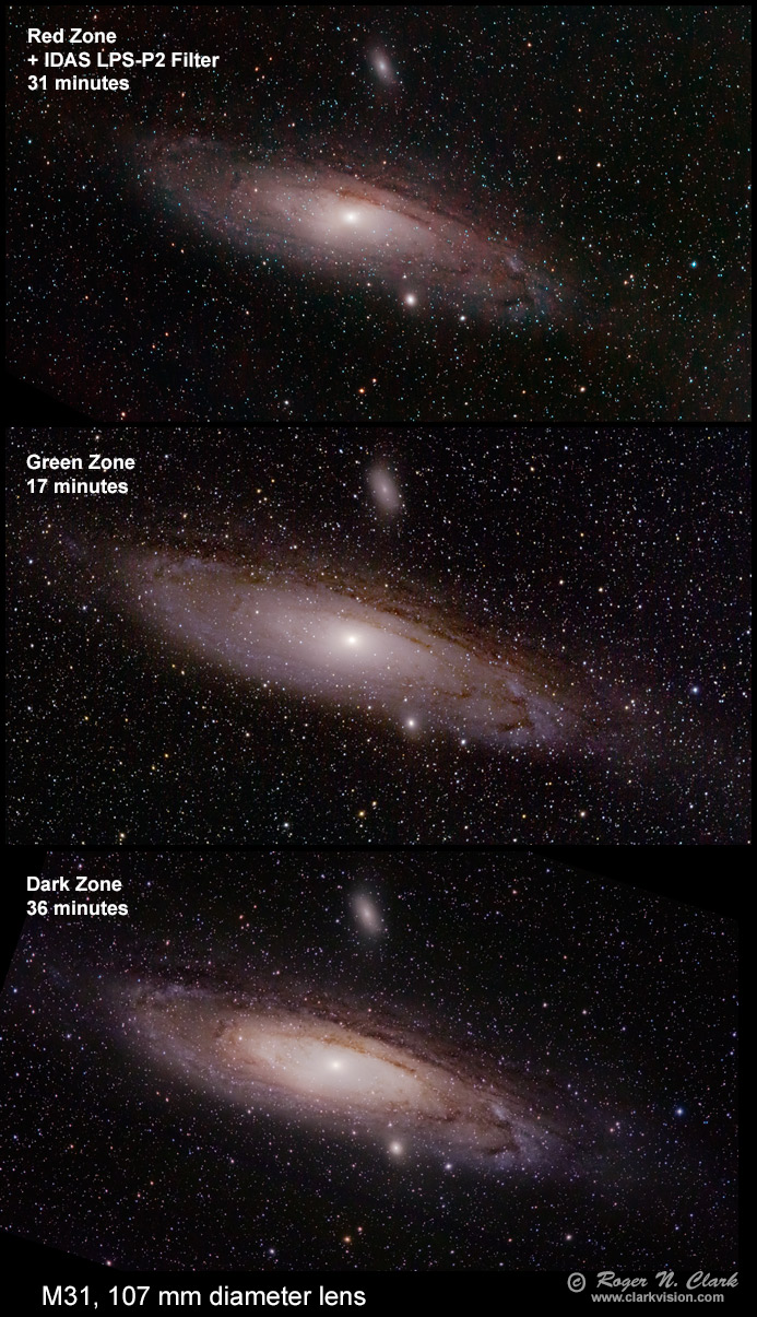
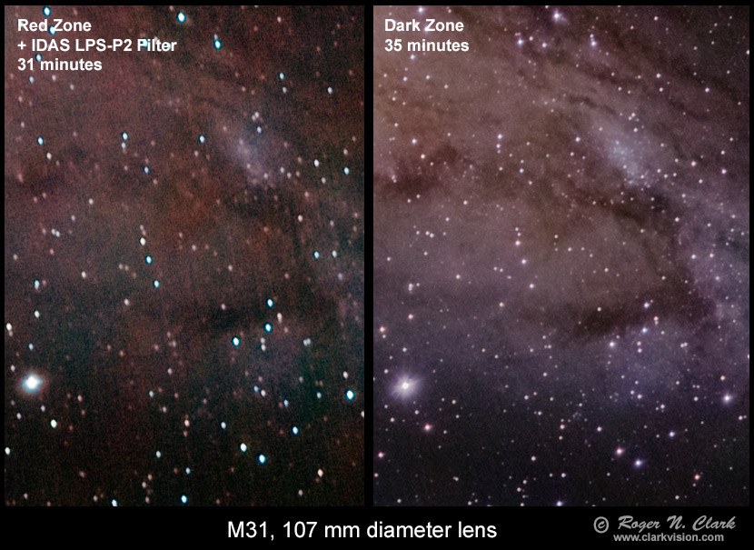
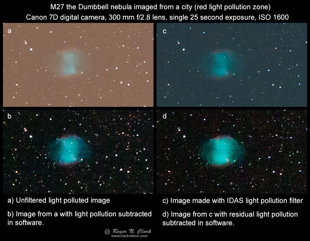
Example images with effects of light pollution are shown in Figures 9a ad 9b. The images were made in a red zone, green zone and at a very dark site (dark gray zones on light pollution maps) and processed to produce the best image I could. All were made with the same 107 mm diameter lens. The red and green zone images were made with a Canon 7D mark 1 with 4.3 micron pixels. The dark zone image was made with a 7D Mark 2 with 4.09 micron pixels which has a better sensor, but the main effects shows here are dominated by effects from light pollution.
Compare the images in Figure 9a and 9b. In 9a, the light pollution was extremely bright, even with the light pollution rejection filter used. The high light pollution, which was subtracted, meant difficulty in establishing a very uniform background, leading to the red-blue splotchiness seen in Figure 9b, left panel. The dark site, which had some airglow that needed to be subtracted, produced a much smoother and more uniform color. I had to spend a lot more time on the red zone image to subtract the background and control color balance. Images made through the IDAS LPS-P2 filter come out very blue with daylight white balance. In the raw converter, one can set a custom white balance of about 7600 Kelvin with tint in ACR around +35. Those setting gave a relative neutral color to solar-type stars in my case. Another example is shown in Figure 9c.
By examining the CEF and CEFA values for the various exposures, some general guidelines can be derived. I base this not only on these images, but the many other astrophotos that I have made with recent model digital cameras.
First, for plate scales in the couple of arc-seconds per pixel range, which matches typical resolution limited by atmospheric turbulence (seeing), CEF values 100 to few hundred range will get to levels that can be seen visually in large telescopes from dark sites. These levels can be achieved from sites 30 to 50 miles from the center of large metropolitan centers of a 2 to 3 million people (green to blue zones on light pollution maps). CEF values in the 1000+ range improves signal-to-noise ratio and brings fainter subjects into view. I strive for CEF in the 2000 to 3000 range, though 3000 to 4000 is better. Some very faint nebulae and galaxies can benefit from CEF levels of 6000 or more.
When comparing diverse resolution imaging, use CEFA. CEFA in the 700+ range records levels that can be observed visually in large amateur telescopes. But 10,000 to 20,000 is needed to image faint objects in high resolution.
For example, images made with a 35 mm f/1.4 lens on a camera with 5.7 micron pixels and 30 second exposures have CEF = 2.45 With 33.6 arc-seconds per pixel, CEFA = 2770, so a little better than the CEFA in Figure 3. But a nightscape made with a 15 mm f/2.8 lens, 30 second exposure would only have a CEF = 0.11, 78.4 arc-seconds per pixel, and CEFA = 693. This says the 35 mm f/1.4 lens will record significantly fainter details.
The CEF and CEFA indicators above are based on reasonably dark skies, blue and green zones on light pollution maps. For sites with more light pollution, additional exposure is needed. In general, for every doubling of sky brightness, exposure factors must increase about 4 times to reach the same faintness.
Credible images can be made in areas of strong light pollution, however, it is difficult to get as faint, it takes more processing to subtract the light pollution well and it can be difficult maintaining a good color balance. The extreme stretched needed in high light pollution environments result in magnification of camera non-uniformities, further degrading the final image quality. Obviously, image quality improves with dark sites with less light pollution, but with careful processing, one can record somewhat faint objects in the night sky even in areas of strong light pollution.
There are other factors than simply exposure time in producing a detailed, low artifact astrophoto. Choosing sub-exposure length for good efficiency, yet allowing one to reject periods of bad seeing, wind gusts, tracking errors, or bumping the system is more important than simply stacking every frame measured in an effort to maximize signal-to-noise ratio. In other words, bad data in, bad data out. Don't let a few exposures with bad image quality contaminate many high quality images in order to maximize signal-to-noise ratio.
Finally, be wary of internet "experts" who say you need to expose for hours to get great images. Gee, people made great images on film with an hour or so exposure time, and film is 20 and more times less sensitive than modern digital cameras! It didn't take days to get great images on film, and it doesn't take hours with digital cameras. The metric, as we have seen above, is not simply exposure time. It is CEF and CEFA. Also, be wary of internet "experts" who say your sub-exposure times are too short and you would do better with longer sub exposures, especially when your exposure times are in a good region of the sub-exposure efficiency model above.
References and Further Reading
Clarkvision.com Astrophoto Gallery.
Clarkvision.com Nightscapes Gallery.
Notes:
DN is "Data Number." That is the number in the file for each pixel. It is a number from 0 to 255 in an 8-bit image file, 0 to 65535 in a 16-bit unsigned integer tif file.
16-bit signed integer: -32768 to +32767
16-bit unsigned integer: 0 to 65535
Photoshop uses signed integers, but the 16-bit tiff is unsigned integer (correctly read by ImagesPlus).
The Night Photography Series:
| Home | Galleries | Articles | Reviews | Best Gear | Science | New | About | Contact |
http://www.clarkvision.com/articles/astrophotography.and.focal.length
First Published January 4, 2016
Last updated October 12, 2021